Chapter 3 Vectors

3.1 Coordinate Systems 3.2 Vector & Scalar Quantities 3.3 Properties of Vectors 3.4 Components of a Vector & the Unit Vector

3.5 Properties of dot products                 (cross products covered in Ch 11)             i.e. Lagrange’s formula             a x (bxc) = b(a ● c) – c(a ●b) 3.6 3.7   Relative Velocities

3.1 Coordinate Systems

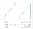
Cartesian (rectangular) to Polar coordinates. It appears the Rigorous method is definitely easier since the formulas NEVER change. The point of view method yields rx =    r sinθ ry = - r cosθ So whether to use cosine or sine depends on the angle that is given. The point of view method requires thought & sketches, instead of just memorization (which at best causes vectors to be incorrect by 180°, 50% of the time.) Not convincing enough???  Just wait.

1st Quadrant Vector

Point of View rx =   r cosθ ry =   r sinθ

Rigorous rx = r cosφ ry = r sinφ

2nd Quadrant Vector

rx = - r cosθ ry =    r sinθ

rx = r cosφ ry = r sinφ

3rd Quadrant Vector

rx = - r cosθ ry = - r sinθ

rx = r cosφ ry = r sinφ

4th Quadrant Vector

rx =    r cosθ ry = - r sinθ

rx = r cosφ ry = r sinφ

Active Figure 3.2                                Active Figure 3.3

3.2 Vectors & Scalar Quantities & 3.3 Properties of Vectors

Definitions Scalar à Magnitude only (is completely specified by a single value with an appropriate unit and has no direction.) Vector à Magnitude with direction (is completely specified by a number and appropriate units plus a direction)

Example: Scalar à Distance drove to school Vector à Distance and direction to come to school

Active Figure 3.6

3.4 Components of a vector & the unit vector

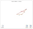
Treasure Hunting in the Islands. You have found a treasure map. a. You must start at the Big Island b. From the Big Island travel 8 mile due North c. At this point you must turn West and travel for 5 miles d. Now travel SW for 6 miles At this point you should find the treasure. Graphical Method

Vector

Rx

Ry

Analytical Method Vector A has no component in the horizontal direction. All is vertical and positive. Vector B has no component in the vertical direction. All is horizontal and negative. Vector C is below

A

0

4

B

-2.5

0

C

3(-cos45) = -2.1

3(-sin45) = -2.1

E

Ex

Ey

0

0

Summation of X components

0 – 2.5 – 2.1 + Ex = 0

Ex = 4.6 miles

Summation of Y components

4 + 0 – 2.1 + Ey = 0

Ey = - 1.9 miles At this point ALWAYS sketch the equilibrant  vector

Direction of Equilibrant Vector

tan θ = oppo / adj tan θ = 1.9 / 4.6 θ = 22.4° South of East

Magnitude of Equilibrant Vector

a^2     + b^2 = c^2 4.6^2 + 1.9^2        = |E|^2 |E| = 5.0 miles

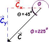
Think About It Now if we ignore everything and use the Rigorous Method we have tan θ = oppo / adj tan θ = -1.9 / 4.6 θ = - 22.4° Which is IDENTICAL to the Point of View perspective θ = 22.4° South of East So why do I say that you will make a mistake 50% of the time using the Rigorous method w/o drawing pictures? See Below   à

Think About It Point 1

Point of View Method

Ex = - 4.6 ; Ey = - 1.9

tan θ = oppo / adj tan θ = 1.9 / 4.6         θ = 22.4° South of West

Rigorous Method

tan θ = - 1.9 / - 4.6         θ = 22.4°

22.4° is NOT in the 3^rd Quadrant, thus w/o a picture to show you that it’s (22.4° past 180°) or 202.4°; this is WRONG!

Think About It Point 2

Point of View Method

Ex = - 4.6 ; Ey = + 1.9

tan θ = oppo / adj tan θ = 1.9 / 4.6         θ = 22.4° North of West

Rigorous Method

tan θ = + 1.9 / - 4.6         θ = - 22.4° or 337.6°

337.6° is NOT in the 2^nd Quadrant, thus w/o a picture to show you that it’s at 157.6° (180° out of phase); this is WRONG!

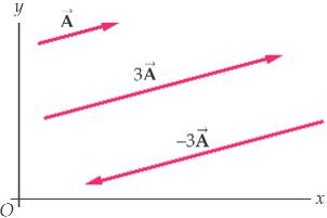
Unit vectors are dimensionless vectors of unit length.

Multiplying unit vectors by scalars: the multiplier changes the length, and the sign indicates the direction.

Active Figure 3.16                                 Demo:  Vector Addition:  ME-A-VE

3.4 Dot Products

a●b = |a| |b| cosθ a●a = a^2 (r1a) ● b = r1(a●b) = a ● (r1 b )  (also see below, scalar multiplication) a●b = Σa1b1 + a2b2 + a3b3 + … anbn

Example 1 (2D) (1,2) ● (4,5) = 1(4) + 2(5) (1,2) ● (4,5) = 14 This can also be written in unit vector notation ( 1 i +  2 j ) ● ( 4 i + 5 j ) = 14

Example 2 (3D) (1,2,3) ● (4,5,6) = 1(4) + 2(5) + 3(6) (1,2,3) ● (4,5,6) = 32 This can also be written in unit vector notation ( 1 i + 2 j + 3 k ) ● ( 4 i + 5 j + 6 k ) = 32

The dot product assumes that are a, b, c, d are vectors and r is scalar.

Commutative a●b = b●a

Bilinear a●(rb + c) = r(a●b) + a●c

Two non-zero vectors a and b are orthogonal if and only if a⋅b = 0.

Distributive  a●(b + c) = a●b + a●c

Scalar multiplication (r1a)●(r2b) = r1r2 (a●b)

If a●b = a●c and a ≠ 0, then we can write: a ● (b − c) = 0 This just means that a is perpendicular to (b − c), which still allows (b − c) ≠ 0, and therefore b ≠ c. If a and b are functions, then the derivative of a ● b is a'●b + a●b'

Cosine Law c●c = (a – b) ● (a – b) c●c = a ● (a – b) - b ● (a – b) c●c = a●a -  a●b -  b●a +  b●b c^2   =   a^2   - a●b -  b●a +   b^2 c^2   =   a^2   - 2a●b + b^2 c^2   =   a^2 + b^2 - 2ab cosθ

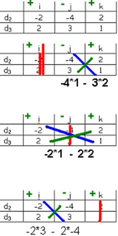
Example 3 all in SI units d1 = -5.2 i + 4.2 j + 3.8 k d2 = -2 i   – 4 j    + 2k d3 = 2i     + 3 j    + 1k

(a)    d1 ● (d2 + d3)         d1 ● [(-2+2)i + (-4+3)j + (2 +1)k]               d1             ●   [ 0 i + -1 j + 3 k]         (-5.2i + 4.2j + 3.8k) ● (0i -1j + 3k)         -5.2*0 + 4.2*(-1) + 3.8*3         7.2 m^2

(d2  X d3)

(b)  d1 ● (d2  X d3) Step 1              (d2  X d3) +[-4*1 – 3*2] i – [-2*1 – 2*2] j + [-2*3 – 2*-4] k +[-10] i –     [-6] j +      [2] k d2  X d3 = -10i + 6j + 2k Step 2          d1                   ●     (d2  X d3) (-5.2i + 4.2j + 3.8k) ●     (d2  X d3) (-5.2i + 4.2j + 3.8k) ● (-10i + 6j + 2k) -5.2*-10  +  4.2*6   +  3.8*2    52        + 25.2      + 7.6 d1 ● (d2  X d3) = 84.8 m^3

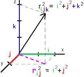
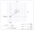
Example A vector is given by R = 2i + j + 3k.  Find (a) the magnitudes of the x, y, and z components, (b) the magnitude of R, and (c) the angles between R & the x, y, & z axes. Note unit vector bx = (1,0,0), also read as x hat
a)       just simply state the coefficients for the x, y, & z components:  2, 1, 3	b )  see figure à r^2 = i^2 + j^2 + k^2 r = (2^2 + 1^2 + 3^2)^1/2           r = 3.74
c)       cos ax = r×bx / |r||b| bx = ( 1, 0, 0 ) cos ax = 2 / |3.74||1| ax = 57.7°	cos ay = r×by / |r||b| by = ( 0, 1, 0 ) cos ay = 1 / |3.74||1| ay = 74.5°						cos az = r×bz / |r||b| bz = ( 0, 0, 1 ) cos az = 3 / |3.74||1| az = 36.7°
3.6 Position, Displacement, Velocity, and Acceleration Vectors
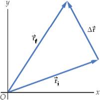
Position vectors ri and rf point from the origin to the location in question at different times. And Δr is the displacement vector pointing from the initial position to the final position.
vave = Δr / Δt Also the resultant position vector is in the same direction.
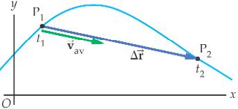
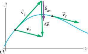
As discussed in lecture, the instantaneous velocity vector is the tangent line to the path. And the change of velocity is the vector between the initial and final velocity vectors.
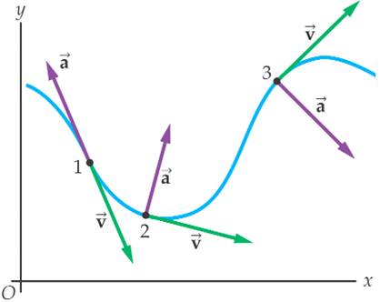
This introduces us to Chapter 4 (Radial Acceleration) and Chapter 5 (Newton’s 2^nd Law) An acceleration either changes speed, OR causes a curve (radial acceleration) if the force is applied inward (as seen to the right) The velocity vector at any point is simply tangential to any point along the curve.
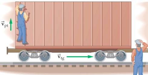
3.7 Relative Motion
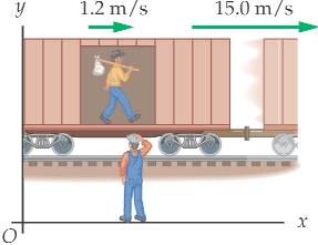
15 + 1.2 = 16.2 m/s It appears the hobo in the train car is moving +16.2 m/s from the train engineer’s perspective
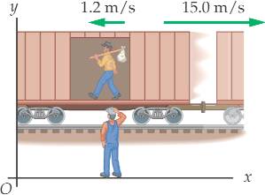
15 – 1.2 = 13.8 m/s It appears the hobo in the train car is moving +13.8 m/s from the train engineer’s perspective
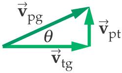
a^2 + b^2 = c^2 or             vtg^2 + vpt^2 = vpg^2
Example A ball of mass 0.2 kg has a velocity of 1.50 i m/s; a ball of mass 0.3 kg has a velocity of -0.4 i m/s.  They meet in a head-on collision.  (a) Find their velocities after the collision.  (b) Find the velocity of their center of mass before and after the collision.
Use relative velocities from ch 4 If v1 = 1.5 and v2 = -0.4 then It appears to v1 that v2 is approaching at 1.9 m/s as if v1 is not moving.		v1   -  1.5   = 0 v2   + 0.4   = 0  (subtract the two equations) v1 - v2 -1.9 = 0                          or   v1 = 1.9 + v2 This is before collision After the collision, it is reversed                         v2f = 1.9 + v1f
m1   v1       + m2    v2 = m1f   v1f +  m2f v2f 0.2*1.5     + 0.3*(-.4)        = 0.2 * v1f         +  0.3 v2f Use relative velocities from section 4.6 v1-init = 1.9 + v2-init   then  v2f = 1.9 m/s + v1f 0.2*1.5     + 0.3*(-.4)        = 0.2 * v1f         + 0.3(1.9 m/s + v1f) 0.3           - 0.12               = 0.2v1f     + 0.57 + 0.3v1f 0.3           - 0.12               = 0.5v1f     + 0.57 v1f    = -0.78 m/s v2f    = 1.12 m/s This gives you a hint of the fun we will be encountering in Chapter 9						(b) vCM = (m1fv1f + m2fv2f)   / m vCM = 0.2*1.5 + 0.3*(-4)/5 vCM = +0.36 m/s This is vCM before the collision…and since momentum is conserved, this is also the vCM after the collision.